Reflection waveform inversion
Conventional FWI has problems updating the deeper part of the model when the recorded data has insufficient diving wave information. As an alternative flavour to FWI, Reflection waveform inversion (RWI) seeks to harness the reflection data that extend to the deepest reflectors to overcome the diving-wave limitation of standard FWI. In RWI, the waveform inversion problem is re-formulated by explicitly separating the (velocity) model reconstruction into two processes: a low-wavenumber background reconstruction and a high-wavenumber reflectivity update. The reflectivity is retrieved by an LSM algorithm and used as a prior (initial guess) for the background model updates. The background model reconstruction uses a weak tomography-like transmission component built with a reflection kernel (the rabbit-ears wave paths). This kernel does not consider the stronger migration isochrone on the conventional FWI sensitivity kernel, which is useless for macro velocity model building and imprints a mispositioned seismic image into the reconstruction.
RWI sensitivity kernel
In this section, I calculate the sensitivity kernel (gradient for a single source-receiver pair) of the reflection waveform inversion problem for a toy experiment using the acoustic wave equation with constant density inspired by Operto (slides 161-166). Operto shows his results in the frequency domain. I follow his notation for simplicity, but my implementation and results are in the time-domain.
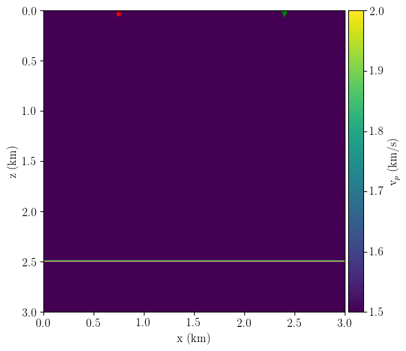
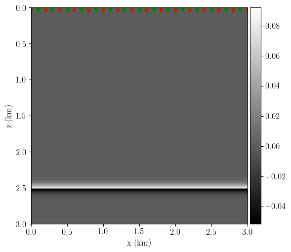
The experiment setup consists of one single source-receiver pair at the surface of a homogeneous 2D velocity field with a single horizontal reflector, as shown in Figure 1. In RWI, the background velocity and reflectivity reconstruction are done alternatingly (expensive!). However, the reflectivity model is assumed to be known to show the RWI sensitivity kernel in this example.
Following Operto (slide 163), the linearized RWI cost function is written as \[\begin{equation} C(\mathbf{m}) = \frac{1}{2}||\delta \mathbf{d}(\mathbf{m}) - \delta\mathbf{d}_{\text{obs}} ||_2^2, \end{equation}\] with \(\mathbf{m}\) denoting the parametrization of the low-wavenumber subsurface velocity model in terms of the squared slowness, \(\delta\mathbf{d}_{\text{obs}}\) represents the observed reflection data, \(\mathbf{P}\) is a “sample at the receiver position” or extraction operator such that \(\delta\mathbf{d}(\mathbf{m}) = \mathbf{P}\delta\mathbf{u}(\mathbf{m})\), and \(\delta\mathbf{u}(\mathbf{m})\) is the modeled scattered data that satisfies the wave equation under the Born approximation, \[ \mathbf{A}(\mathbf{m})\delta \mathbf{u} = -\omega^2\text{diag}(\delta \mathbf{m})\mathbf{u}(\mathbf{m})\tag{2}, \] where \(\delta\mathbf{m}\) is the high-wavenumber reflectivity component, \(\mathbf{u}\) is the down-going source wavefield, and \(\mathbf{A}(\mathbf{m})= \Big[\omega^2\text{diag}(\mathbf{m}) + \nabla \Big]\).
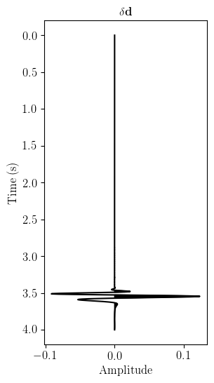
For this toy problem, Figure 2 shows the observed reflection data recorded at the receiver position using a Ricker wavelet of 10 Hz as the seismic source.
In the frequency domain, the adjoint-state method permits to express the gradient of the RWI function as (the derivation using Lagrange multipliers is on Operto’s slides):
\[\begin{align*} \nabla_\mathbf{m} C &= \mathcal{R}\Big\{{\Big(\frac{\partial\mathbf{A}(\mathbf{m})}{\partial\mathbf{m}}\mathbf{u}\Big)^T\bar{\mathbf{a}}_1}\Big\} + \mathcal{R}\Big\{{\Big(\frac{\partial\mathbf{A}(\mathbf{m})}{\partial\mathbf{m}}\delta\mathbf{u}\Big)^T\bar{\mathbf{a}}_2}\Big\}\\ &= \omega^2 \sum_\omega\mathcal{R}\{\mathbf{u}^T\bar{\mathbf{a}}_1 + \delta \mathbf{u}^T \bar{\mathbf{a}}_2 \}\tag{3}, \end{align*}\]
where \(\bar{\mathbf{a}}_1\) and \(\bar{\mathbf{a}}_2\) are two adjoint wavefields satisfying \[\begin{align*} \mathbf{A}^T(\mathbf{m})\bar{\mathbf{a}}_2&=\mathbf{P}^T(\delta\mathbf{d}(\mathbf{m}) - \delta \mathbf{d}_{\text{obs}}),\tag{4}\\ \mathbf{A}^T(\mathbf{m})\bar{\mathbf{a}}_1&=\omega^2\text{diag}(\delta \mathbf{m})\bar{\mathbf{a}}_2,\tag{5} \end{align*}\] and \(\mathbf{P}^T\) denotes the “inject at the receiver position” operator (adjoint of the extraction).
Equivalently, in the time-domain: \[ \begin{equation*}\tag{6} \nabla_\mathbf{m} C = \sum_t \Big(\mathbf{u}(t)\frac{\partial^2\mathbf{a}_1(t)}{\partial t^2} + \delta\mathbf{u}(t)\frac{\partial^2\mathbf{a}_2(t)}{\partial t^2} \Big). \end{equation*} \]
Things to consider
Equation 4 describes the computation of the well-known back-propagated receiver wavefield from RTM/LSRTM/FWI workflows: use the reflection data as the adjoint source and inject them at the receiver(s) position backwards in time to generate \(\bar{\mathbf{a}}_2\). (See next section)
Comparing equations 2 and 5, we can see that the relation between source-wavefield and scattered wavefield, \(\mathbf{u}\) and \(\delta\mathbf{u}\), is the same as the back-propagated receiver wavefield and the second adjoint wavefield, \(\bar{\mathbf{a}}_2\) and \(\bar{\mathbf{a}}_1\). One is in the contrast source (right-hand-side) of the other. The main difference is that equation 2 is computed in forward mode and equation 5 in backward mode. This is excellent because I can recycle my codes from RTM/LSM/FWI with minimal modifications.
Backward perturbation field \(\mathbf{a}_1\)
I cannot stress the previous point enough! It is critical to understand how to form the reflection-based tomographic kernel. People familiarized with classic RTM/LSM/FWI recognize the other three wavefields: \(\mathbf{u}, \delta\mathbf{u}\) and \(\mathbf{a}_2\). On the other hand, \(\mathbf{a}_1\) is the backward perturbation field, which is calculated by born modelling of the perturbated reflectivity \(\delta\mathbf{m}\) and the background wavefield \(\mathbf{a}_2\).
- To discuss with MDS: there is also a minus-sign difference in the contrast sources (right-hand sides) of equations 2 and 5. This comes from the lagrangian formulation (equation 183 in Operto’s slides). However, Kryvohuz et al. (2019) has no such a difference. My current implementation also uses the same signs for both equations.
Result
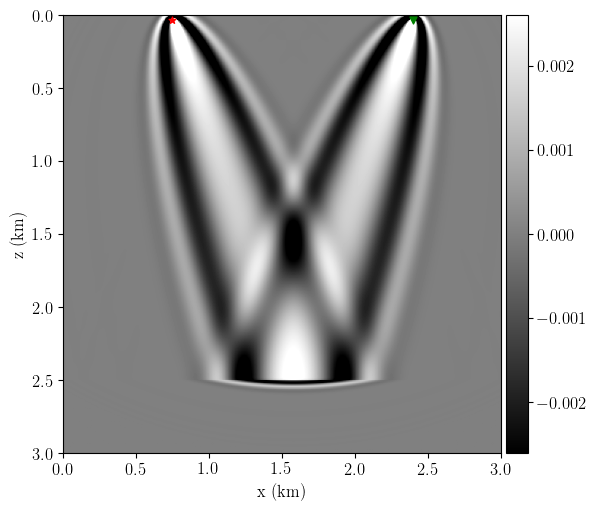
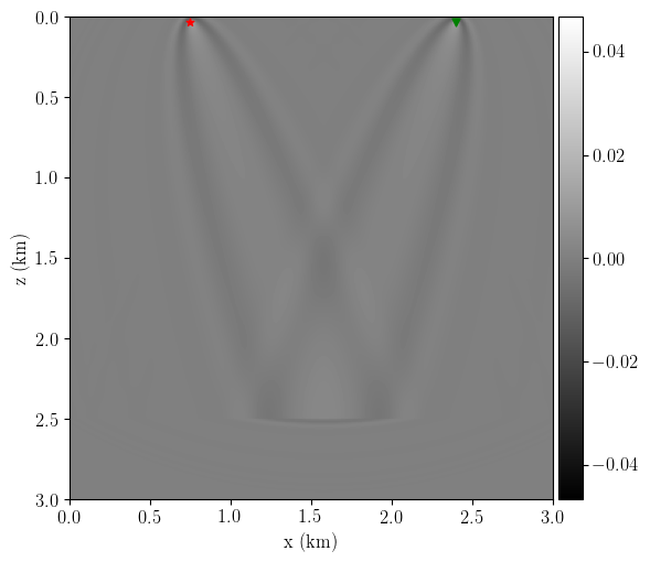
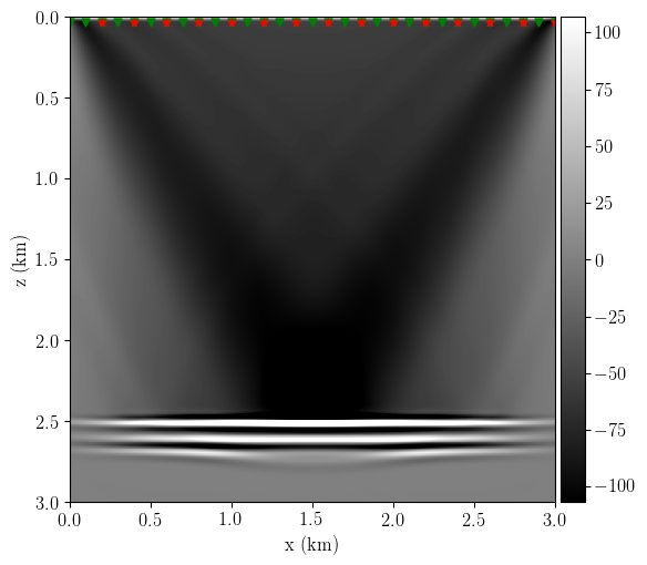
Figure 3 shows the toy experiment’s RWI gradient (equation 3). We can see the distinctive rabbit-ears wave paths and the absence of the banana and migration kernels from standard FWI (see next section).
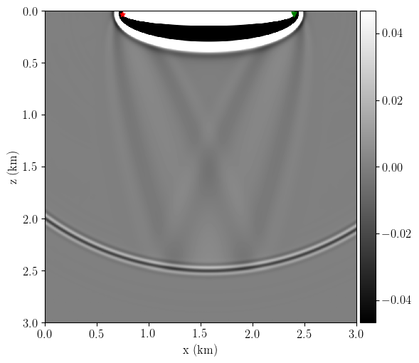
Even though I just said that I only need to store two wavefields to calculate the RWI gradient, to gain some intuition, I save all four wavefields below to show the movie of the sensitivity kernel construction at different time steps (Figure 4).
Comparison with the standard FWI gradient
The standard FWI gradient is \[ \nabla_\mathbf{m} C = \omega^2 \sum_\omega\mathcal{R}\{ u^Ta_2\}\tag{7}. \]
A naive implementation of equation 7 in the time-domain requires that I have access to both wavefields at all times to compute the gradient: \[\begin{equation*}\tag{8} \nabla_\mathbf{m} C = \sum_t \mathbf{u}(t)\frac{\partial^2\mathbf{a}_2(t)}{\partial t^2}. \end{equation*}\]
One can also compute the source-wavefield \(\mathbf{u}\) first and store it (either in memory or disk), and then accumulate the dot-product (zero-lag cross-correlation, imaging condition) between wavefields at each time-step while computing the adjoint wavefield backwards in time. This way, I only need to store one of the two required wavefields (although practitioners use more advanced techniques to reduce the wavefield storage burden).
Similarly, in my current implementation of the RWI gradient, I only need to store two wavefields: \(\mathbf{u}\) and \(\delta\mathbf{u}\). So, I first compute a forward Born modelling that saves these two fields (source-wavefield and scattered-wavefield) and then use them as inputs, along with the estimated reflectivity model \(\delta\mathbf{m}\), and the observed data \(\delta\mathbf{d}\), to compute the two adjoint wavefields (equations 4 and 5) while performing on-the-fly (and accumulating) the zero-lag cross-correlations of the two terms in equation 3 at each time-step. No adjoint wavefield is stored anywhere as in standard RTM/LSRTM/FWI.
Finally, Figure 5 compares the kernels between standard FWI and RWI for the same toy setup. The rabbit ears in the standard FWI gradient are barely noticeable compared to the stronger banana and migration kernels.
RWI updates for multiple sources and receivers
Extending the RWI gradient calculation to several sources and receivers is trivial. In this section, I simulate a full-acquisition RWI inversion step. This example illustrates how the RWI gradient provides information about low-wavenumber velocity updates from mismatches between observed and synthetic data.
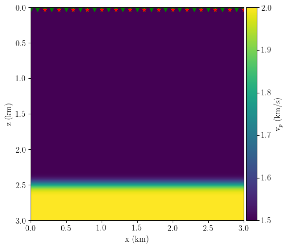
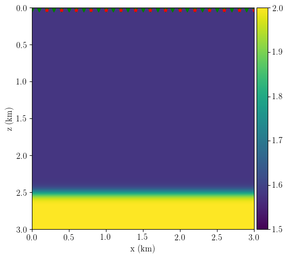
The experiment setup changes slightly concerning the previous example: now, the true model is a smoothed version of a two-layered media \(v_{p1}=1.5\) km/s, \(v_{p2} = 2\) km/s with the velocity contrast at z=2.50 km. I use this true model to generate the observed data with 400 sources and 400 receivers evenly distributed at the surface. Next, I define my initial smooth velocity model with 5% faster velocity on the first layer. I also set the initial reflectivity (used to generate the synthetic data) by changing the depth of the velocity contrast to z=2.52 km. Figure 6 shows the experiment setup.
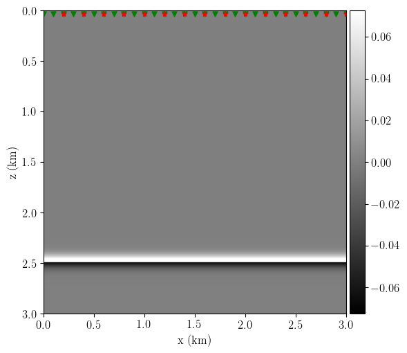
Figure 7 shows the RWI low-wavenumber velocity update, where I obtain the correct update direction, i.e., dark colours indicating a slow down on the first layer with 5% faster velocity. There is also a higher wavenumber component due to the mismatch in the depth of the velocity contrast from the true and initial reflectivity models.
Next steps
Operto says: “When the reflectivity is generated, its position in depth is such that simulated zero-offset traveltimes in the background velocity model (demigration step) match the recorded ones.” Gomes and Chazalnoel (2017) make the same claim: “Because the reflector depth is self-derived from each initial model, both tests match the observed data at zero-offset.” How is this possible? I think they are referring to the fact that after some velocity update iterations with the residuals, the derived model will tend to match the observed data even if the inversion goes to a local minimum.
This is an initial step into the understanding of RWI, but now that I can compute its gradient, I could perform RWI by incorporating my LSM code into this framework.

References
Gomes, A, and N Chazalnoel. 2017. “Extending the Reach of FWI with Reflection Data: Potential and Challenges.” In 79th EAGE Conference and Exhibition 2017-Workshops, cp–519. EAGE Publications BV.
Kryvohuz, Maksym, Henning Kuehl, René-Édouard Plessix, and Yi Yang. 2019. “Reflection Full-Waveform Inversion with Data-Space LSRTM.” In SEG Technical Program Expanded Abstracts 2019, 1229–33. Society of Exploration Geophysicists.